In the last post we looked at how Generative Adversarial Networks could be used to learn representations of documents in an unsupervised manner. In evaluation, we found that although the model was able to learn useful representations, it did not perform as well as an older model called DocNADE. In this post we give a brief overview of the DocNADE model, and provide a TensorFlow implementation.
![fvsbn]()
![nade]()
One additional change from the evaluation in the paper is that we evaluate the average perplexity over the full test set (in the paper they just take a random sample of 50 documents).
We were expecting to see an improvement due to the use of the full softmax, but not an improvement of quite this magnitude. Even when using a sampled softmax on this task instead of the full softmax, we see some big improvements over the published results. This suggests that the hierarchical softmax formulation that was used in the original paper was a relatively poor approximation of the true softmax (but it’s possible that there is a bug somewhere in our implementation, if you find any issues please let us know).
We also see an improvement on the document retrieval evaluation results with the full softmax:
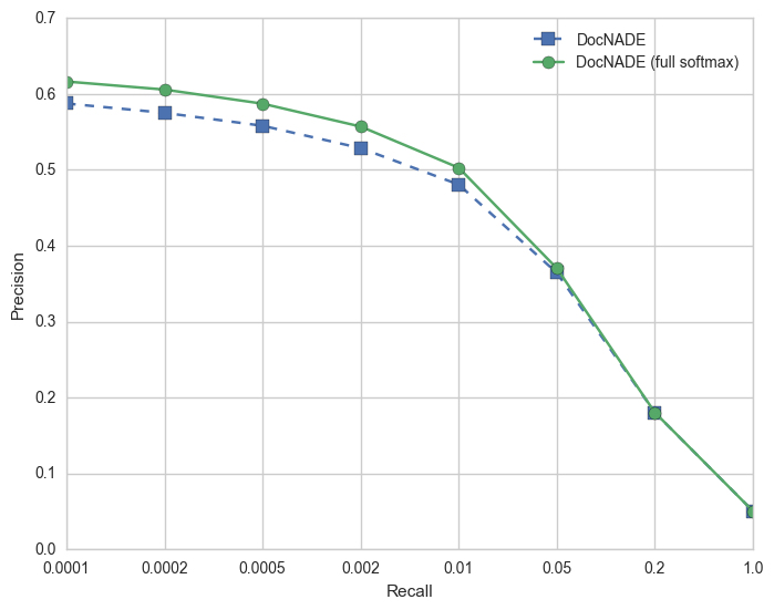
For the retrieval evaluation, we first create vectors for every document in the dataset. We then use the held-out test set vectors as “queries”, and for each query we find the closest N documents in the training set (by cosine similarity). We then measure what percentage of these retrieved training documents have the same newsgroup label as the query document. We then plot a curve of the retrieval performance for different values of N. Note: for working with larger vocabularies, the current implementation supports approximating the softmax using the sampled softmax.
Neural Autoregressive Distribution Estimation
Recent advances in neural autoregressive generative modeling has lead to impressive results at modeling images and audio, as well as language modeling and machine translation. This post looks at a slightly older take on neural autoregressive models - the Neural Autoregressive Distribution Estimator (NADE) family of models. An autoregressive model is based on the fact that any D-dimensional distribution can be factored into a product of conditional distributions in any order:\(p(\mathbf{x}) = \prod_{d=1}^{D} p(x_d | \mathbf{x}_{<d})\)
where \(\mathbf{x}_{<d}\) represents the first \(d-1\) dimensions of \(\mathbf{x}\) in the current ordering. We can therefore create an autoregressive generative model by just parameterising all of the separate conditionals in this equation. One of the more simple ways to do this is to take a sequence of binary values, and assume that the output at each timestep is just a linear combination of the previous values. We can then pass this weighted sum through a sigmoid to get the output probability for each timestep. This sort of model is called a fully-visible sigmoid belief network (FVSBN):A fully visible sigmoid belief network. Figure taken from the NADE paper.
Here we have binary inputs \(v\) and generated binary outputs \(\hat{v}\). \(\hat{v_3}\) is produced from the inputs \(v_1\) and \(v_2\). NADE can be seen as an extension of this, where instead of a linear parameterisation of each conditional, we pass the inputs through a feed-forward neural network:Neural Autoregressive Distribution Estimator. Figure taken from the NADE paper.
Specifically, each conditional is parameterised as:\(p(x_d | \mathbf{x_{<d}}) = \text{sigm}(b_d + \mathbf{V}_{d,:} \mathbf{h}_d)\)
\(\mathbf{h}_d = \text{sigm}(c + \mathbf{W}_{:,<d} \mathbf{x}_{<d})\)
where \(\mathbf{W}\), \(\mathbf{V}\), \(b\) and \(c\) are learnable parameters of the model. This can then be trained by minimising the negative log-likelihood of the data. When compared to the FVSBN there is also additional weight sharing in the input layer of NADE: each input element uses the same parameters when computing the various output elements. This parameter sharing was inspired by the Restricted Boltzmann Machine, but also has some computational benefits - at each timestep we only need to compute the contribution of the new sequence element (we don’t need to recompute all of the preceding elements).Modeling documents with NADE
In the standard NADE model, the input and outputs are binary variables. In order to work with sequences of text, the DocNADE model extends NADE by considering each element in the input sequence to be a multinomial observation - or in other words one of a predefined set of tokens (from a fixed vocabulary). Likewise, the output must now also be multinomial, and so a softmax layer is used at the output instead of a sigmoid. The DocNADE conditionals are then given by:\(p(x | \mathbf{x_{<d}}) = \frac{\text{exp} (b_{w_d} + \mathbf{V}_{w_d,:} \mathbf{h}_d) } {\sum_w \text{exp} (b_w + \mathbf{V}_{w,:} \mathbf{h}_d) }\)
\(\mathbf{h}_d = \text{sigm}\Big(c + \sum_{k<d} \mathbf{W}_{:,x_k} \Big)\)
An additional type of parameter sharing has been introduced in the input layer - each element will have the same weights no matter where it appears in the sequence (so if the word “cat” appears input positions 2 and 10, it will use the same weights each time). There is another way to look at this however. We now have a single set of parameters for each word no matter where it appears in the sequence, and there is a common name for this architectural pattern - a word embedding. So we can view DocNADE a way of constructing word embeddings, but with a different set of constraints than we might be used to from models like Word2Vec. For each input in the sequence, DocNADE uses the sum of the embeddings from the previous timesteps (passed through a sigmoid nonlinearity) to predict the word at the next timestep. The final representation of a document is just the value of the hidden layer at the final timestep (or in the other words, the sum of the word embeddings passed through a nonlinearity). There is one more constraint that we have not yet discussed - the sequence order. Instead of training on sequences of words in the order that they appear in the document, as we do when training a language model for example, DocNADE trains on random permutations of the words in a document. We therefore get embeddings that are useful for predicting what words we expect to see appearing together in a full document, rather than focusing on patterns that arise due to syntax and word order (or focusing on smaller contexts around each word).An Overview of the TensorFlow code
The full source code for our TensorFlow implementation of DocNADE is available on Github, here we will just highlight some of the more interesting parts. First we do an embedding lookup for each word in our input sequence (x). We initialise the embeddings to be uniform in the range [0, 1.0 / (vocab_size * hidden_size)], which is taken from the original DocNADE source code. I don’t think that this is mentioned anywhere else, but we did notice a slight performance bump when using this instead of the default TensorFlow initialisation.
with tf.device('/cpu:0'):
    max_embed_init = 1.0 / (params.vocab_size * params.hidden_size)
    W = tf.get_variable(
        'embedding',
        [params.vocab_size, params.hidden_size],
        initializer=tf.random_uniform_initializer(maxval=max_embed_init)
    )
    self.embeddings = tf.nn.embedding_lookup(W, x)
tf.scan function to apply sum_embeddings to each sequence element in turn. This replaces each embedding with sum of that embedding and the previously summed embeddings.
def sum_embeddings(previous, current):
    return previous + current

h = tf.scan(sum_embeddings, tf.transpose(self.embeddings, [1, 2, 0]))
h = tf.transpose(h, [2, 0, 1])

h = tf.concat([
    tf.zeros([batch_size, 1, params.hidden_size], dtype=tf.float32), h
], axis=1)

h = h[:, :-1, :]
bias = tf.get_variable(
    'bias',
    [params.hidden_size],
    initializer=tf.constant_initializer(0)
)
h = tf.tanh(h + bias)
h = tf.reshape(h, [-1, params.hidden_size])
logits = linear(h, params.vocab_size, 'softmax')
loss = masked_sequence_cross_entropy_loss(x, seq_lengths, logits)
Experiments
As DocNADE computes the probability of the input sequence, we can measure how well it is able to generalise by computing the probability of a held-out test set. In the paper the actual metric that they use is the average perplexity per word, which for time \(t\), input \(x\) and test set size \(N\) is given by:\(\text{exp} \big(-\frac{1}{N} \sum_{t} \frac{1}{|x_t|} \log p(x_t) \big)\)
As in the paper, we evaluate DocNADE on the same (small) 20 Newsgroups dataset that we used in our previous post, which consists of a collection of around 19000 postings to 20 different newsgroups. The published version of DocNADE uses a hierarchical softmax on this dataset, despite the fact that they use a small vocabulary size of 2000. There is not much need to approximate a softmax of this size when training relatively small models on modern GPUs, so here we just use a full softmax. This makes a large difference in the reported perplexity numbers - the published implementation achieves a test perplexity of 896, but with the full softmax we can get this down to 579. To note how big an improvement this is, the following table shows perplexity values on this task for models that have been published much more recently:| Model/paper | Perplexity |
| DocNADE (original) | 896 |
| Neural Variational Inference | 836 |
| DeepDocNADE | 835 |
| DocNADE with full softmax | 579 |
For the retrieval evaluation, we first create vectors for every document in the dataset. We then use the held-out test set vectors as “queries”, and for each query we find the closest N documents in the training set (by cosine similarity). We then measure what percentage of these retrieved training documents have the same newsgroup label as the query document. We then plot a curve of the retrieval performance for different values of N. Note: for working with larger vocabularies, the current implementation supports approximating the softmax using the sampled softmax.
Conclusion
We took another look a DocNADE, noting that it can be viewed as another way to train word embeddings. We also highlighted the potential for large performance boosts with older models due simply to modern computational improvements - in this case because it is no longer necessary to approximate smaller vocabularies. The full source code for the model is available on Github.Related Content
-
 General
20 Aug, 2024
The advantage of monitoring long tail international sources for operational risk

Keith Doyle
4 Min Read
-
General
16 Feb, 2024
Why AI-powered news data is a crucial component for GRC platforms

Ross Hamer
4 Min Read
-
General
24 Oct, 2023
Introducing Quantexa News Intelligence
Ross Hamer
5 Min Read
Stay Informed
From time to time, we would like to contact you about our products and services via email.