From July 20th to July 28th 2016, I had the opportunity of  attending the 6th Lisbon Machine Learning School. The Lisbon Machine Learning School (LxMLS) is an annual event that brings together researchers and graduate students in the fields of NLP and Computational Linguistics, computer scientists with an interest in statistics and ML, and industry practitioners with a desire for a more in-depth understanding. Participants had a chance to join workshops and labs, where they got hands-on experience with building and exploring state-of-the-art deep learning models, as well as to attend talks and speeches by prominent deep learning and NLP researchers from a variety of academic and industrial organisations. You can find the entire programme here. In this blog post, I am going to share some of the highlights, key insights and takeaways of the summer school. I am going to skip the lectures of the first and second day as they introduce basic Python, Linear Algebra, and Probability Theory concepts and focus on the later lectures and talks. First, we are going to talk about sequence models. We will then turn to structured prediction, a type of supervised ML common to NLP. We will then summarize the lecture on Syntax and Parsing and finally provide insights with regard to Deep Learning. The accompanying slides can be found as a reference at the end of this blog post. Disclaimer: This blog post is not meant to give a comprehensive introduction of each of the topics discussed; it should rather give you an overview of the week-long event and provide you with pointers if you want to delve deeper into any of the topics.

Sequence Models

Noah Smith of the University Washington kicked off the third day of the summer school with a compelling lecture about sequence models. To test your understanding of sequence models, try to answer – without reading further – the following question: What is the most basic sequence model depicted in Figure 1?

Figure 1: The most basic sequence model

Correct! It is the bag-of-words (notice which words have “fallen” out of the bag-of-words). The bag-of-words model makes the strongest independence assumption of all sequence models: It supposes that each word is entirely independent of its predecessors. It is obvious why models that rely on this assumption do only a poor job at modelling language: every word naturally depends on the words that have preceded it. Somewhat more sophisticated models thus relax this naive assumption to reduce the entropy: A 1st Order Markov model makes each word dependent on the word that immediately preceded it. This way, it is already able to capture some context of the context that can help to disambiguate a new word. More generally, (m^{ ext{th}}) Order Markov Models make each word depend on its previous (m) words. In mathematical terms, in (m^{ ext{th}}) Order Markov Models, the probability of a text sequence (we assume here that such a sequence is delimited by start and stop symbols) can be calculated using the chain rule as the product of the probabilities of the individual words: (p( ext{start}, w_1, w_2, …, w_n, ext{stop}) = prodlimits_{i=1}^{n+1} gamma (w_i : | : w_{i-m}, …, w_{i-1}) ) where (gamma) is the probability of the current word (w_i) given its (m) previous words, i.e. the probability to transition from the previous words to the current word. We can view bag-of-words and (m^{ ext{th}}) Order Markov Models as occupying the following spectrum:

Figure 2: From bag-of-words to history-based models

As we go right in Figure 2, we make weaker independence assumption and in exchange gain richer expressive power, while requiring more parameters – until we eventually obtain the most expressive – and most rigid – model, a history-based model where each word depends on its entire history, i.e. all preceding words. As a side-note, state-of-the-art sequence modelling models such as recurrent neural networks and LSTMs can be thought of as being located on the right side of this spectrum, as they don’t require an explicit specification of context words but are – theoretically – able to take into account the entire history. In many cases, we would not only like to model just the observed sequence of symbols, but take some additional information into account. Hidden Markov Models (HMMs) allow us to associate with each symbol (w_i) some missing information, its “state” (s_i). The probability of a word sequence in an HMM then not only depends on the transition probability (gamma) but also on the so-called emission probability (eta): (p( ext{start}, w_1, w_2, …, w_n, ext{stop}) = prodlimits_{i=1}^{n+1} eta (w_i : | : s_i) : gamma (s_i : | : s_{i-1}) ) Consequently, the HMM is a joint model over observable symbols and hidden/latent/unknown classes. HMMs have traditionally been used in part-of-speech tagging or named entity recognition where the hidden states are POS and NER tags respectively. If we want to determine the most probable sequence of hidden states, we face a space of potential sequences that grows exponentially with the sequence length. The classic dynamic algorithm to cope with this problem is the Viterbi algorithm, which is used in HMMs, CRFs, and other sequence models to calculate the most probable sequence of hidden states: It lays out the symbol sequence and all possible states in a grid and proceeds left-to-right to compute the maximum probability to transition in every new state given the previous states. The most probable sequence can then be found by back-tracking as in Figure 3.

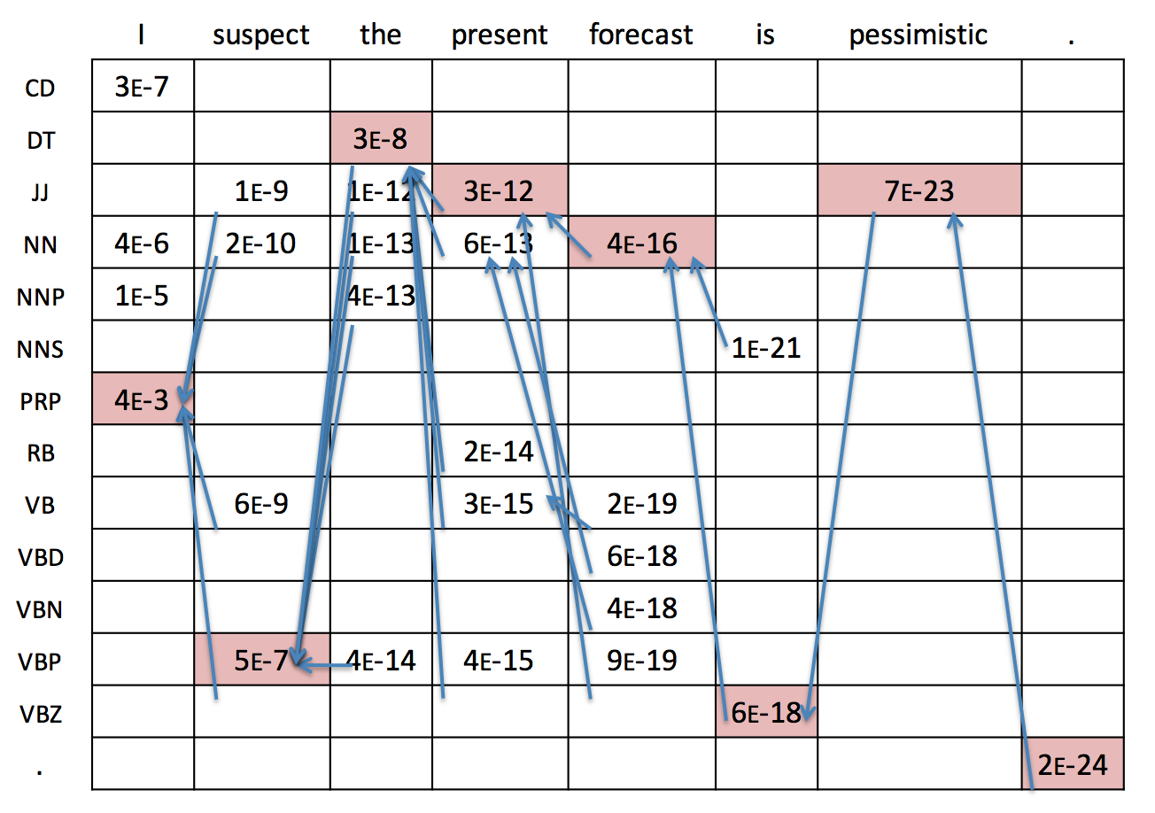
Figure 3: The Viterbi algorithm

A close relative is the forward-backward algorithm, which is used to calculate the probability of a word sequence and the probabilities of each word’s states, e.g. for language modelling. Indeed, the only difference between Viterbi and the forward-backward algorithm is that Viterbi takes the maximum of the probabilities of the previous state, while forward-backward takes the sum. In this sense, they correspond to the same abstract algorithm, which is instantiated in two different semirings where a semiring informally is a set of values and some operations that obey certain properties. Finally, if we want to learn HMMs in an unsupervised way, we use the well-known Expectation Maximisation (EM) algorithm, which consists of two steps: During the E step, we calculate the probability of each possible transition and emission at every position with forward-backward (or Viterbi for “hard” EM); for the M step, we re-estimate the parameters with MLE.

Machine Translation

On the evening of the third day, Philipp Koehn, one of the pioneers of MT and inventor of phrase-based machine translation gave a talk on Machine Translation as Sequence Modelling, including a detailed review of different MT and alignment approaches. If you are interested in a comprehensive history of MT that takes you from IBM Model 1 all the way to phrase-based, syntax-based and eventually neural MT, while delving into the details of alignment, translation, and decoding, definitely check out the slides here.

Structured Prediction

HMMs can model sequences, but as their weights are tied to the generative process, strong independence assumptions need to be made to make their computation tractable. We will now turn to a category of models that are more expressive and can be used to predict more complex structures: Structured prediction -- which was introduced by Xavier Carreras of Xerox Research on the morning of the fourth day -- is used to refer to ML algorithms that don’t just predict scalar or real values, but more complex structures. As complex structures are common in language, so is structured prediction; example tasks of structured prediction in NLP include POS tagging, named entity recognition, machine translation, parsing, and many others. A successful category of structured prediction models are log-linear models, which are so-called because they model log-probabilities using a linear predictor. Such models try to estimate the parameters (w) by calculating the following probability: ( ext{log} : ext{Pr}(mathbf{y} : | : mathbf{x}; mathbf{w}) = ext{log} :rac { ext{exp}{mathbf{w} cdot mathbf{f}(mathbf{x},mathbf{y})}}{Z(mathbf{x};mathbf{w})}) where (mathbf{x} = x_1, x_2, …, x_n in mathcal{X}) is the sequence of symbols, (mathbf{y} = y_1, y_2, …, y_n in mathcal{Y}) is the corresponding sequence of labels, (mathbf{f}(mathbf{x},mathbf{y})) is a feature representation of (mathbf{x}) and (mathbf{y}), and (Z(mathbf{x};mathbf{w}) = sumlimits_{mathbf{y}’ in mathcal{Y}} ext{exp}(mathbf{w} cdot mathbf{f}(mathbf{x},mathbf{y}’)) ) is also referred to as the partition function. Two approaches that can be used to estimate the model parameters (w) are:

1. Maximum Entropy Markov Models (MEMMs), which assume that ( ext{Pr}(mathbf{y} : | : mathbf{x}; mathbf{w})) decomposes, i.e. that we can express it as a product of the individual label probabilities that only depend on the previous label (similar to HMMs).
2. Conditional Random Fields (CRFs), which make a weaker assumption by only assuming that (mathbf{f}(mathbf{x},mathbf{y})) decomposes.

In MEMMs, we assume – similarly to Markov Models – that the label (y_i) at the (i) th position does not depend on all past labels, but only on the previous label (y_{i-1}). In contrast to Markov Models, MEMMs allow us to condition the label (y_i) on the entire symbol sequence (x_{1:n}). Both assumptions combined lead to the following probability of label (y_i) in MEMMs: ( ext{Pr}(y_i : | : x_{1:n}, y_{1:i-1}) = ext{Pr}(y_i : | : x_{1:n}, y_{i-1})) By this formulation, the objective of MEMMs reduces sequence modelling to multi-class logistic regression. In CRFs, we factorize on label bigrams. Instead of greedily predicting the most probable label (y_i) at every position (i), we instead aim to find the sequence of labels with the maximum probability: (underset{y in mathcal{Y}}{ ext{argmax}} sum_i mathbf{w} cdot mathbf{f}(mathbf{x}, i, y_{i-1}, y_i)) We then estimate the parameters (w) of our model using gradient-based methods where we can use forward-backward to compute the gradient.

CRFs vs. MEMMs

By choosing between MEMMs and CRFs, we make the choice between local and global normalisation. While MEMMs aim to predict the most probable label at every position, CRFs aim to find the most probable label sequence. This, however, leads to the so-called “Label Bias Problem” in MEMMs: As MEMMs choose the label with the highest probability, the model is biased towards more frequent labels, often irrespective of the local context. As MEMMs reduce to multi-class classification, they are cheaper to train. On the other hand, CRFs are more flexible and thus easier to extend to more complex structures. This distinction between local and global normalisation has been a recurring topic in sequence modelling and a key criterion when choosing an algorithm. For text generation tasks, global normalisation is still too expensive, however. Many state-of-the-art approaches thus employ beam search as a compromise between local and global normalisation. In most sequence modelling tasks, local normalisation is very popular due to its ease of use, but might fall out of favour as more advanced models and implementations for global normalisation become available. To this effect, a recent outstanding paper at ACL (Andor et al., 2016) shows that globally normalised models are strictly more expressive than locally normalised ones.

HMMs vs. CRFs

Another distinction that is worth investigating is the difference between generative and discriminative models: HMMs are generative models, while CRFs are discriminative. HMMs only take into account the previous word as its features are tied to the generative process. In contrast, CRF features are very flexible. They can look at the whole input (x) paired with a label bigram ((y_i , y_{i+1})). In practice, for prediction tasks, such “good” discriminative features can improve accuracy a lot. Regarding the parameter estimation, the distinction between generative and discriminative becomes apparent: HMMs focus on explaining the data, both (x) and (y), while CRFs focus on the mapping from (x) to (y). Which model is more appropriate depends on the task: CRFs are commonly used in tasks such as POS tagging and NER, while HMMs have traditionally lain at the heart of speech recognition.

Structured Prediction in NLP with Imitation Learning

Andreas Vlachos of the University of Sheffield gave a talk on using imitation learning for structured prediction in NLP, which followed the same distinction between local normalisation (aka incremental modelling), i.e. greedily predicting one label at a time and global normalisation (aka joint modelling), i.e. scoring the complete outputs with a CRF that we discussed above. Andreas talked about how imitation learning can be used to improve incremental modelling as it allows to a) explore the search space, b) to address error-propagation, and c) to train with regard to the task-specific loss function. There are many popular imitation learning algorithms in the literature such as SEARN (Daumé III et al., 2009), Dagger (Ross et al. 2011), or V-DAgger (Vlachos and Clark, 2014). Recently, MIXER (Ranzato et al., 2016) has been proposed to directly optimise metrics for text generation, such as BLEU or ROUGE. An interesting perspective is that imitation learning can be seen as inverse reinforcement learning: Whereas we want to learn the best policy in reinforcement learning, we know the optimal policy in imitation learning, i.e. the labels in the training data; we then infer the per-action reward function and learn a policy, i.e. a classifier that can generalise to unseen data.

Demo Day

Figure 4: Aylien stand at Demo Day

In the evening of the fourth day, we presented – along with other NLP companies and research labs – Aylien at the LxMLS Demo Day. We presented an overview of our research directions at Aylien, as well as a 1D generative adversarial network demo and visualization.

Syntax and Parsing

Having looked at generic models that are able to cope with sequences and more complex structures, we now briefly mention some of the techniques that are commonly used to deal with one of language’s unique characteristics: syntax. To this end, Slav Petrov of Google Research gave an in-depth lecture about syntax and parsing on the fifth day of the summer school, which discussed, among others, successful parsers such as the Charniak and the Berkeley parser, context-free grammars and phrase-based parsing, projective and non-projective dependency parsing, as well as more recent transition and graph-based parsers. To tie this to what we’ve already discussed, Figure 5 demonstrates how the distinction between generative and discriminative models applies to parsers.

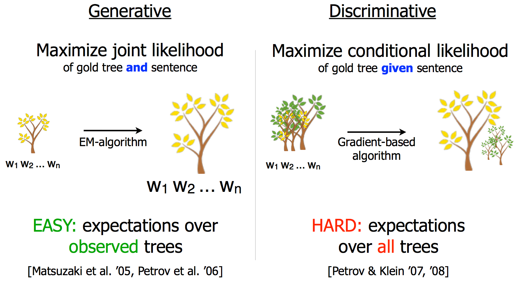Figure 5: Generative vs. discriminative parsing models

From Dependencies to Constituents

In the evening of the fifth day, André Martins of Unbabel gave talk a on an ACL 2015 paper of his, in which he shows that constituent parsing can be reduced to dependency parsing to get the best of both worlds: the informativeness of constituent parser output and the speed of dependency parsers. Their approach works for any out-of-the-box dependency parser, is competitive for English and morphologically rich languages, and achieves results above the state of the art for discontinuous parsing (where edges are allowed to intersect).

Deep Learning

Finally, the two last days were dedicated to Deep Learning and featured prolific researchers from academia and industry labs as speakers. On the morning of the sixth day, Wang Ling of Google DeepMind gave one of the most gentle, family-friendly intro to Deep Learning I’ve seen – titled Deep Neural Networks Are Our Friends with a theme inspired by the Muppets. The evening talk by Oriol Vinyals of Google DeepMind detailed some of his lessons learned when working on sequence-to-sequence models at Google and gave glimpses of interesting future challenges, among them, one-shot learning for NLP (Vinyals et al., 2016) and enabling neural networks to ponder decisions (Graves, 2016). For the lecture on the last day, Chris Dyer of CMU and Google DeepMind discussed modelling sequential data with recurrent neural networks (RNNs) and shared some insights and intuitions with regard to working with RNNs and LSTMs.

Exploding / vanishing gradients

If you’ve worked with RNNs before, then you’re most likely familiar with the exploding/vanishing gradients problem: As the length of the sequence increases, computations of the model get amplified, which leads to either exploding or vanishing gradients and thus renders the model incapable to learn. The intuition why advanced models such as LSTMs and GRUs mitigate this problem is that they use summations instead of multiplications (which lead to exponential growth).

Deep LSTMs

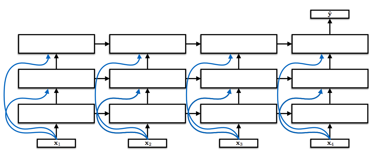Figure 6: Deep LSTMs

Deep or stacked LSTMs are by now a very common sight in the literature and state-of-the-art for many sequence modelling problems. Still, descriptions of implementations often omit details, which might be perceived as self-evident. This, however, means that it is not always clear how a model looks like exactly or how it differs from similar architectures. The same applies to Deep LSTMs. The most standard convention feeds the input not only to the first but (via skip connections) also to subsequent layers as in Figure 6. Additionally, dropout is generally applied only between layers and not on the recurrent connections as this would drop out more and more value over time.

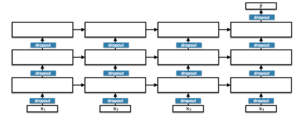Figure 7: Dropout in Deep LSTMs

Does Depth Matter?

Generally, depth helps. However, in comparison to other applications such as audio/visual processing, depth plays a less significant role in NLP. Hypotheses for this observation are: a) More transformation is required for speech processing, image recognition etc. than for common text applications; b) Less effort has been made to find good architectures (RNNs are expensive to train; have been widely used for less long); c) Backpropagation through time and depth is hard and we need better optimisers. Generally, 2-8 layers are standard across text applications. Input skip connections are used often but by no means universally. Only recently have also very deep architectures been proposed for NLP (Conneau et al., 2016).

Mini-batching

Mini-batching is generally necessary to make use of optimised matrix-matrix multiplication. In practice, however, this usually requires bucketing training instances based on similar lengths and padding with (0)'s, which can be a nuisance. Because of this, this is – according to Chris Dyer – “the era of assembly language programming for neural networks. Make the future an easier place to program!”

Character-based models

Character-based models have gained more popularity recently and for some tasks such as language modelling, using character-based LSTMs blows the results of word-based models out of the water, achieving a significantly lower perplexity with a lot fewer parameters particularly for morphologically rich languages.

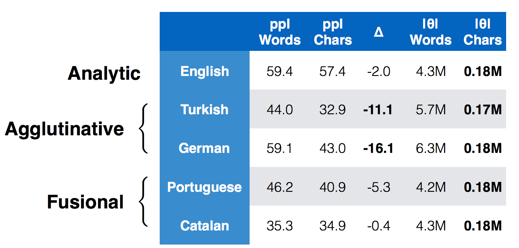Figure 8: CharLSTM > Word Lookup

Attention

Finally, no overview of recurrent neural networks is complete without the mention of attention, one of the most influential, recently proposed notions with regard to LSTMs. Attention is closely related to “pooling” operations in convolutional neural networks (and other architectures) as it also allows to selectively focus on particular elements of the input. The most popular attention architecture pioneered by Bahdanau et al. (2015) seems to only care about “content” in that it relies on computing the dot product, i.e. the cosine similarity between vectors. It contains no obvious bias in favor of diagonals, short jumps, fertility, or other structures that might guide actual attention from a psycho-linguistic perspective. Some work has begun to add other “structural” biases (Luong et al., 2015; Cohn et al., 2016), but there are many more opportunities for research. Attention is similar to alignment, but there are important differences: a) alignment makes stochastic but hard decisions. Even if the alignment probability distribution is “flat”, the model picks one word or phrase at a time; b) in contrast, attention is “soft” (all words are interpolated based on their attention weights). Finally, there is a big difference between “flat” and “peaked” attention weights.

Memory Networks for Language Understanding

Antoine Bordes of Facebook AI Research gave the last talk of the summer school, in which he discussed Facebook AI Research’s two main research directions: On the one hand, they are working on (Key-Value) Memory Networks, which can be used to jointly model symbolic and continuous systems. They can be trained end-to-end through back propagation and with SGD and provide great flexibility on how to design memories. On the other hand, they are working on new tools for developing learning algorithms. They have created several datasets of reasonable sizes, such as bAbI, CBT, and MovieQA that are designed to ease interpretation of a model’s capabilities and to foster research.

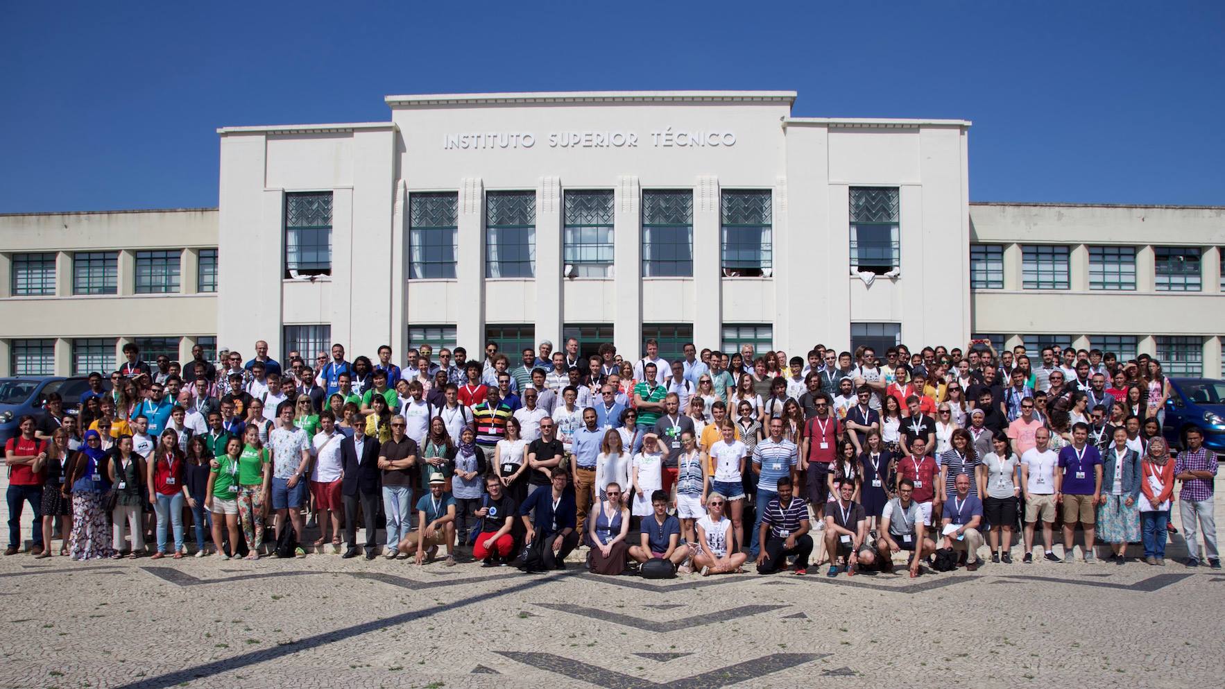Figure 9: LxMLS 2016 Group Picture

That was the Lisbon Machine Learning Summer School 2016! We had a blast and hope to be back next year!

Slides

Sequence Models (Noah Smith) Machine Translation as Sequence Modelling (Philipp Koehn) Learning Structured Predictors (Xavier Carreras) Structured Prediction in NLP with Imitation Learning (Andreas Vlachos) Syntax and Parsing - I, II (Slav Petrov) Turbo Parser Redux: From Dependencies to Constituents (André Martins) Deep Neural Networks Are Our Friends (Wang Ling) Modeling Sequential Data with Recurrent Networks (Chris Dyer) Memory Networks for Language Understanding (Antoine Bordes)